A model can predict flawlessly and have understood nothing
Statistical learning cannot tell you how much data it needs before training, nor whether it learned the law or merely memorised the map. We measure both — and deliver an alternative that is nine orders of magnitude more accurate.
orange = what the law does not contain
What is shown in this dossier is a presentation of measured results. The technology itself is transferred only under an agreed technological cooperation, accepted by all parties involved. What can be made available under such an agreement extends beyond what is presented here.
The two questions training cannot answer
Any model that propagates a state learns a map. The law that generates the map has structure — locality, symmetries, conserved quantities — which the map hides. There is an intrinsic quantity of the problem that simultaneously fixes:
This quantity is computed from the data, before any training. From it follow an exact threshold on the number of examples required, and a test that separates the law from the map.
| What you want to know | Statistical method | Our method |
|---|---|---|
| How much data do I need? | Trial and error | Computed in advance |
| Did I learn the law? | Cannot be known | A four-number certificate |
| Where will it fail? | Test it there | Predicted without testing |
Nothing that follows depends on an architecture choice, a hyperparameter or an initialisation. All figures come from runs against known ground truth.
The number of examples required is exact, not approximate
Same problem, same data, two methods. Direct recovery has a threshold: below it it cannot, at it it knows exactly. The trained network has no threshold at all — it descends smoothly and never reaches precision, not even with twenty times more examples.
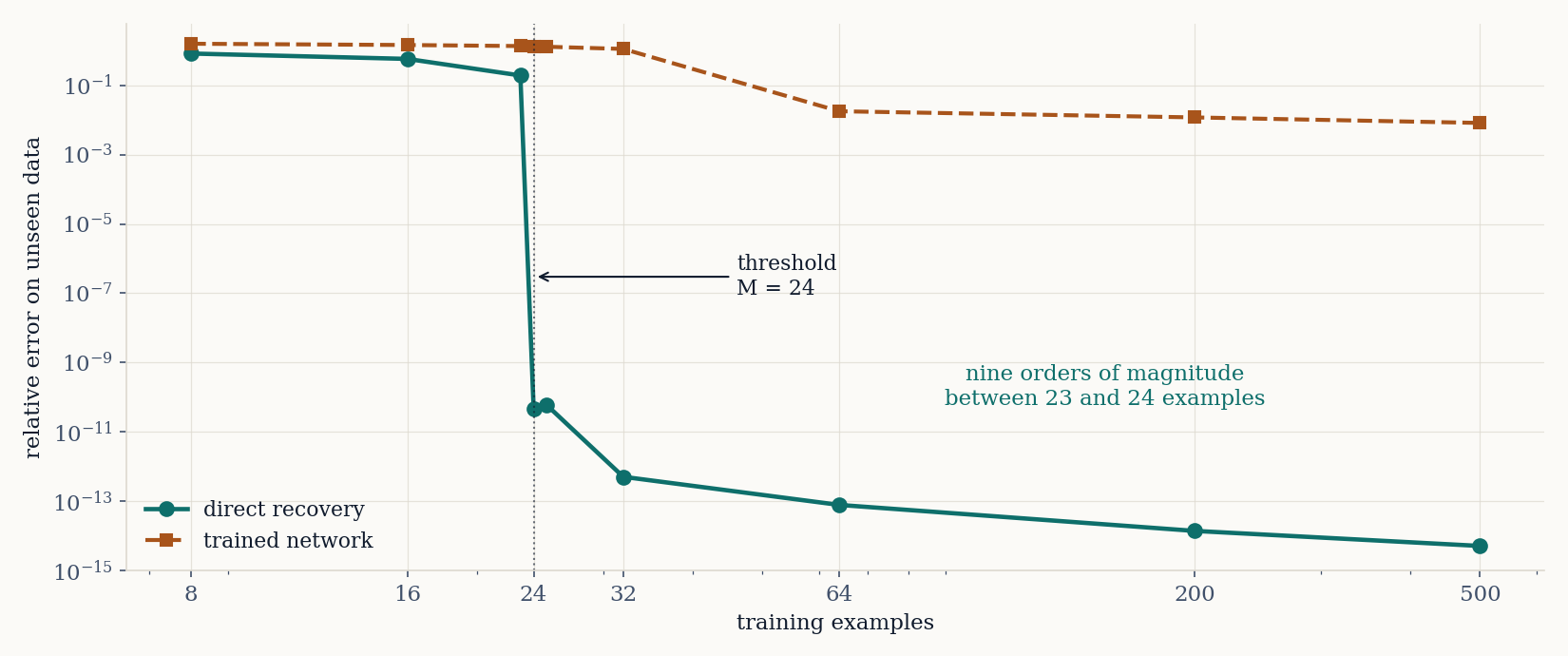
| Examples | Direct recovery | Trained network |
|---|---|---|
| 16 | 5.73×10⁻¹ | 1.44 |
| 23 | 1.91×10⁻¹ | 1.35 |
| 24 | 4.79×10⁻¹¹ | 1.29 |
| 64 | 7.91×10⁻¹⁴ | 1.77×10⁻² |
| 500 | 5.19×10⁻¹⁵ | 8.17×10⁻³ |
Direct consequence. The data-acquisition budget is sized before the first measurement is collected. In applications where a single example is expensive — a physical experiment, a sensor campaign, a high-fidelity simulation — this translates immediately into cost avoided.
A network with good test error and no physics inside
We trained a network to a test error any industrial pipeline accepts. We then measured four structural quantities the test error cannot see, working from the model's behaviour alone. The verdict requires no fresh test set and no access to the model's code.
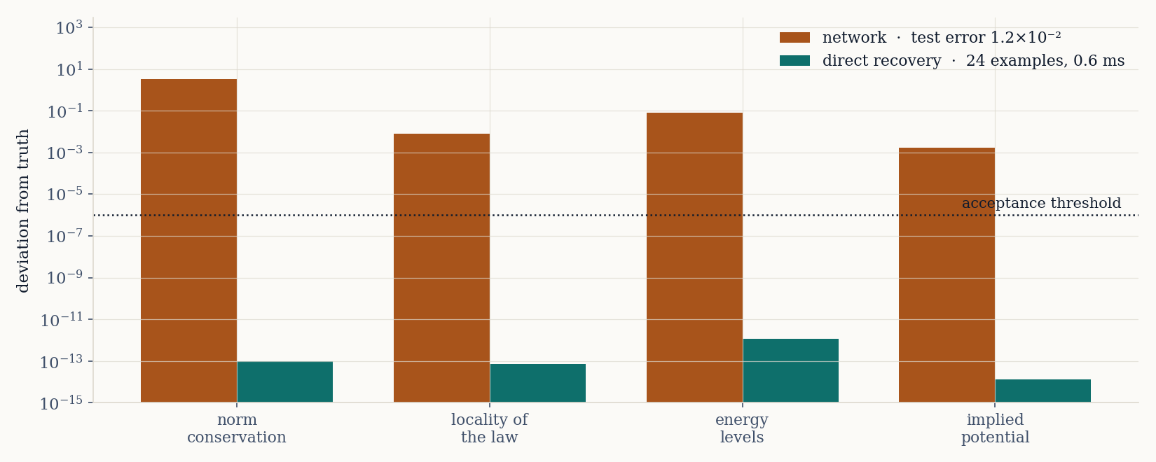
model audited · trained network, 11,664 parameters, 4,000 epochs
test error · 1.25×10⁻² — accepted by any pipeline
structural invariant 1 FAIL (off by a factor of four)
structural invariant 2 FAIL (four orders outside)
structural invariant 3 FAIL (five orders outside)
structural invariant 4 FAIL (four orders outside)
VERDICT NO PHYSICS
reference · direct recovery, 24 examples, 0.6 ms
VERDICT LAW — all four pass
The audit applies to any model that propagates a state — neural operator, simulation surrogate, fluid or climate emulator — and requires no access to its code. Which four quantities, and how they are extracted, is held as trade secret and is communicated within a cooperation.
The physical law emerges from the data; it is not assumed
From short trajectories, with no model assumption, the generating law is recovered. The spatial profile comes out to the thirteenth decimal — including for a fully random law, so no smoothness is being exploited.
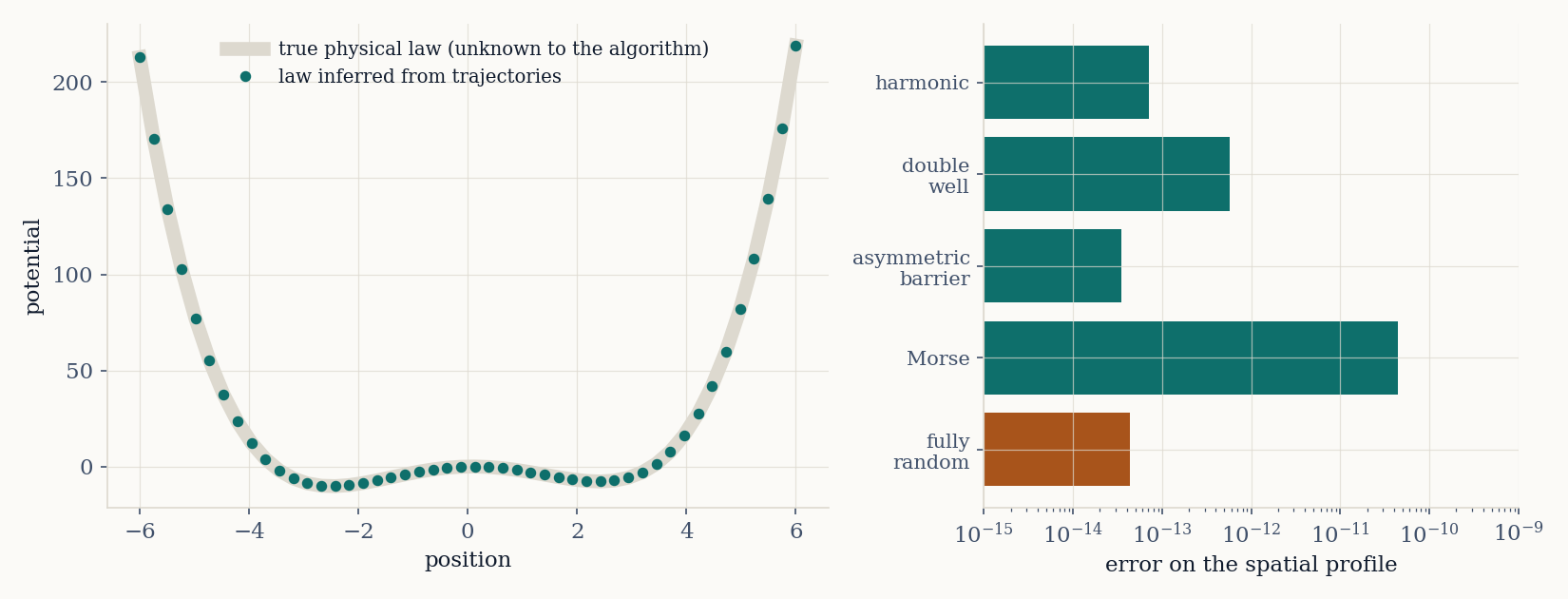
| What was discovered | Error | Note |
|---|---|---|
| Law profile (double well) | 5.7×10⁻¹³ | no model assumed |
| Fully random profile | 4.4×10⁻¹⁴ | no structure to exploit |
| Locality of the interaction | 1.96×10⁻¹³ | was not imposed |
| Topological invariant (flux) | 0.00 | exactly zero error, 169 measurements |
Six tests chosen to break the mechanism — dissipation, a 2D magnetic field, periodically driven systems, nonlinearity, partial observability — were all passed. Where the method does break, it breaks with a measurable signature rather than silently.
Four operations that do not exist in the alternative
A trained model learns a map at one fixed time step. A recovered law is a different object: it propagates to any horizon, at an unseen time step, on states outside the training distribution — and backwards in time. The last one is not “better”; it is impossible for a map learned forward.
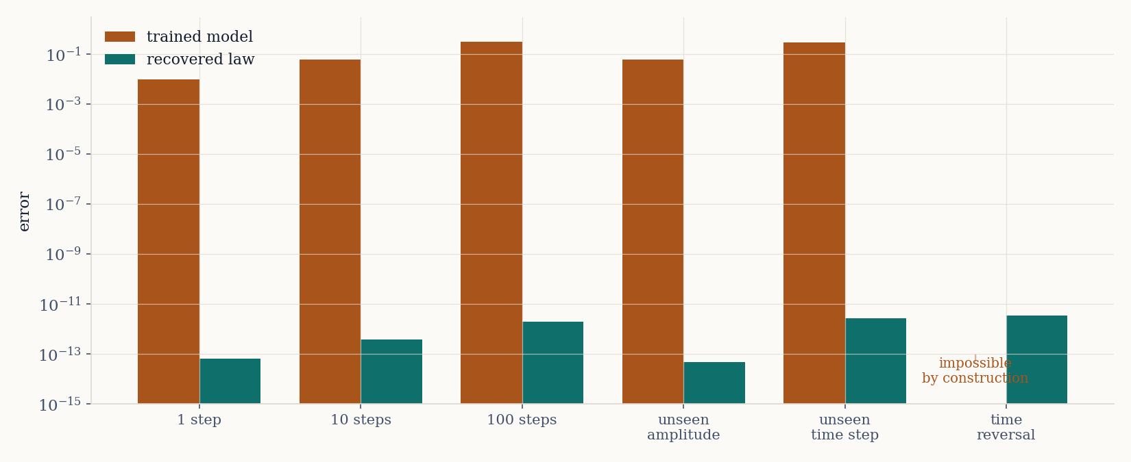
| Task, none seen during training | Trained model | Recovered law | Ratio |
|---|---|---|---|
| Long-horizon propagation (100 steps) | 3.0×10⁻¹ | 1.9×10⁻¹² | 10¹¹ |
| Unseen time step | 2.9×10⁻¹ | 2.7×10⁻¹² | 10¹¹ |
| Out-of-distribution amplitudes | 6.0×10⁻² | 4.6×10⁻¹⁴ | 10¹² |
| Time reversal, and round trip | impossible | 3.5×10⁻¹² | — |
Consequence. A single recovered object covers every operating regime — no model per time step, per horizon, per amplitude regime. The cost of maintaining a family of models disappears.
Two routes with nothing in common reach the same numbers
The physical spectrum was extracted along two independent paths that share no component with one another. Their agreement therefore cannot be a common artefact of either. This is the strongest internal check available to us, and we ran it.
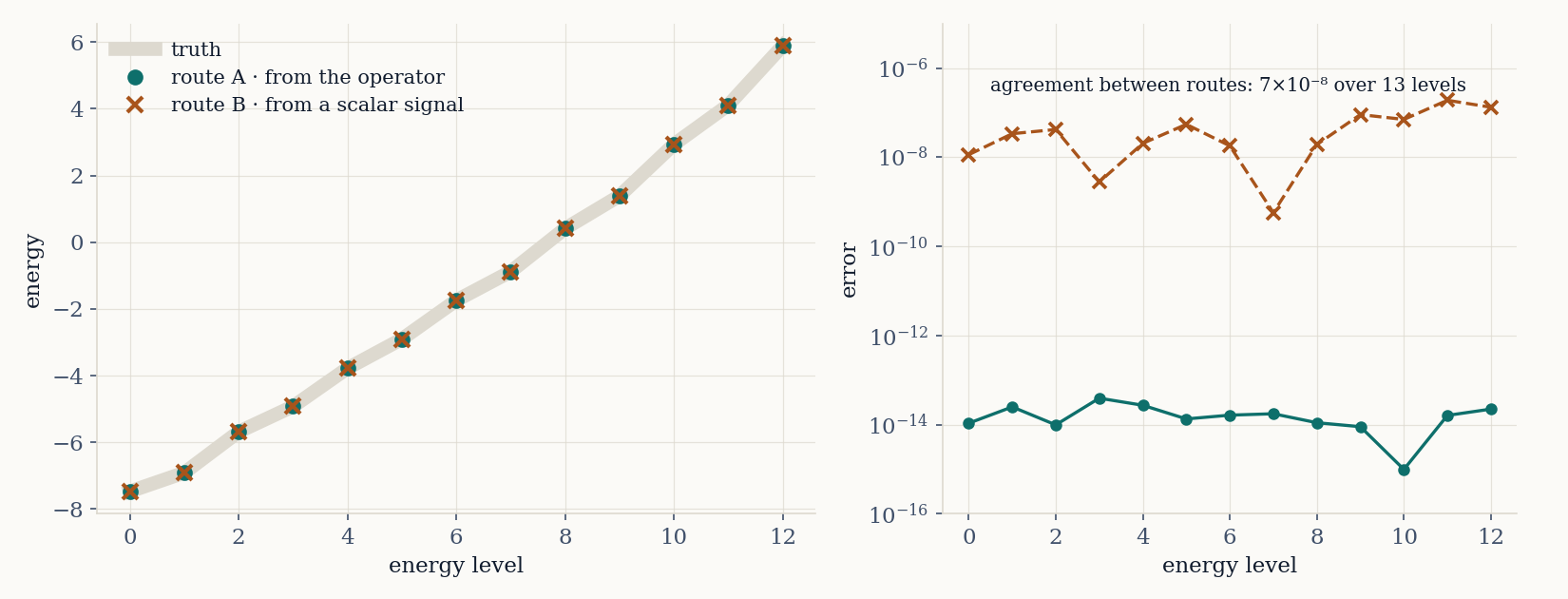
The second route self-limits correctly: it stops exactly where the information required to go further ceases to be present in the data. The limit is one of information, not of method — and the method reports the limit instead of inventing past it.
Five thousand times faster and nine orders more accurate
Same problem, same test data. The middle column is computational effort; the right-hand column is the accuracy reached. The last row is the standard textbook numerical method, which learns nothing from data — included as a reference point.
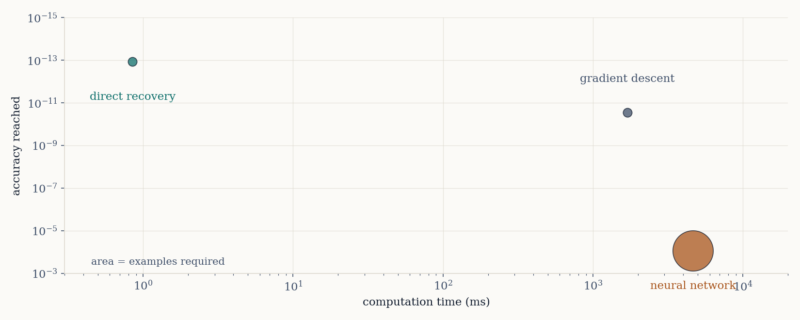
| Method | Examples | Time (ms) | Error |
|---|---|---|---|
| Direct recovery | 24 | 0.85 | 1.19×10⁻¹³ |
| Gradient descent | 24 | 1 696 | 2.83×10⁻¹¹ |
| Trained neural network | 500 | 4 656 | 8.69×10⁻⁵ |
| Standard numerical method (10⁴ steps) | — | — | 1.19 |
The last row deserves separate reading: the standard textbook method, correct by construction, accumulates 1.19 error over ten thousand steps where the recovered law stays at 9×10⁻¹². That is not a comparison against machine learning — it is against current engineering practice.
The reconstruction comes out cleaner than the data it was built from
Counterintuitive, but measured across four decades of noise. The physical parameters do not degrade to the noise level: they come out more than a hundred times more precise. Noise has nowhere to fit inside the representation.
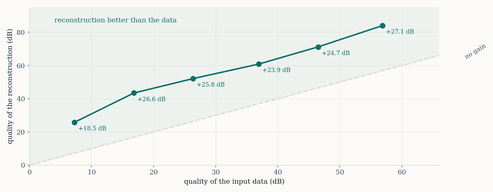
| Input noise | Input quality (dB) | Output quality (dB) | Gain |
|---|---|---|---|
| 30% | 7.3 | 25.8 | +18.5 |
| 10% | 16.8 | 43.4 | +26.6 |
| 1% | 36.9 | 60.9 | +23.9 |
| 0.1% | 56.9 | 84.0 | +27.1 |
Consequence. Sensor quality requirements drop. A measurement chain carrying 10% noise delivers parameters at an accuracy that would normally require a chain a hundred times more expensive.
A system driven a thousand times a second, compressed into a static law
Systems driven by a rapidly oscillating field have no obvious stationary law. From sparsely sampled data, a static description is recovered that characterises them completely. The measured level shift follows the analytic law across three octaves of driving frequency.
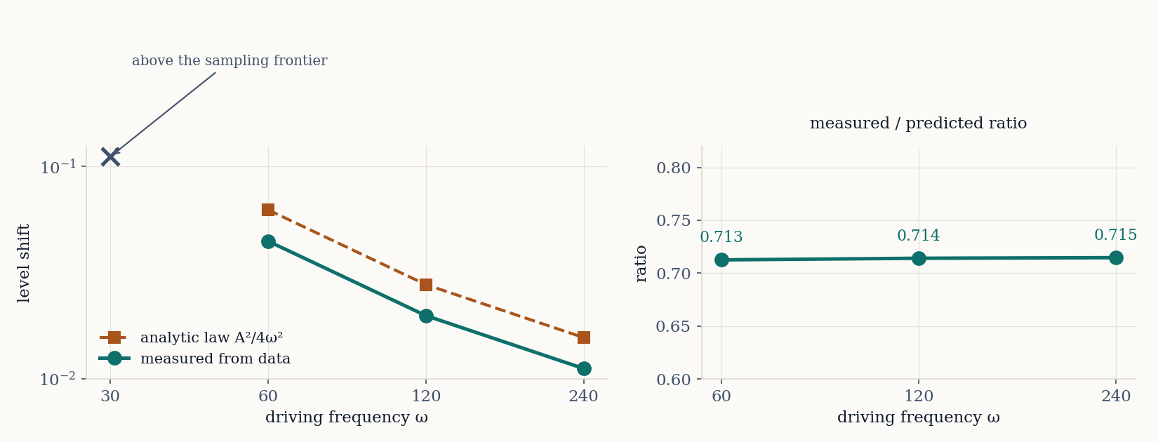
| Frequency ω | Within declared frontier | Measured shift | Analytic law | Non-locality |
|---|---|---|---|---|
| 30 | no | −10.235 | 0.1111 | 4.5×10⁻¹ |
| 60 | yes | 0.04454 | 0.06250 | 4.4×10⁻⁶ |
| 120 | yes | 0.01984 | 0.02778 | 3.8×10⁻⁷ |
| 240 | yes | 0.01117 | 0.01563 | 4.1×10⁻⁸ |
The first row is a deliberate failure. At ω=30 the data falls outside the frontier the method declares for itself, and the recovered law is false — even though the propagator stays exact at 2×10⁻¹⁴. This is the point of the row: the frontier was not tuned after the fact. It predicted the failure before producing it, and we publish the failure rather than the four rows that worked.
When the linear model is not enough, the algorithm states which representation is missing
On a self-interacting system the linear model degrades in proportion to the strength of the nonlinearity — the expected behaviour. Analysis of the residual, however, indicates exactly which representation is required. In that representation the error becomes independent of the nonlinearity's strength.
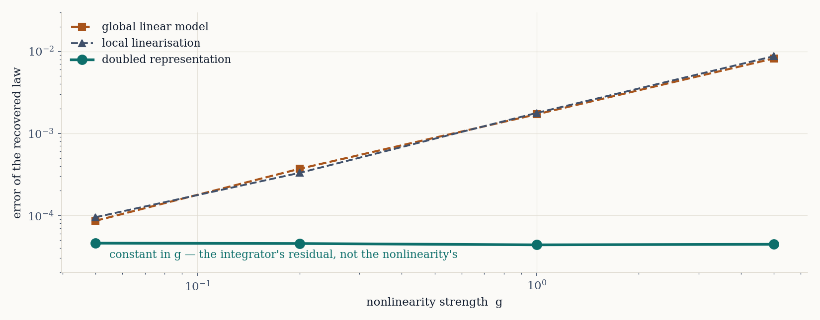
| Nonlinearity strength g | Global linear model | Local linearisation | Indicated representation |
|---|---|---|---|
| 0.05 | 8.57×10⁻⁵ | 9.47×10⁻⁵ | 4.58×10⁻⁵ |
| 0.20 | 3.70×10⁻⁴ | 3.30×10⁻⁴ | 4.53×10⁻⁵ |
| 1.00 | 1.71×10⁻³ | 1.78×10⁻³ | 4.36×10⁻⁵ |
| 5.00 | 8.20×10⁻³ | 8.73×10⁻³ | 4.43×10⁻⁵ |
The last column is constant in g and equal to the error at zero nonlinearity — it is the numerical integrator's residual, not the nonlinearity's. The correct representation came out of the data, not out of theory. A model that merely fails tells you nothing; this one tells you what it lacks.
One hundred thousand steps without drift, on a system that loses energy
Real systems dissipate. The law no longer conserves the norm, and the correct constraint is no longer that of isolated systems. Projecting onto the appropriate constraint keeps propagation stable over horizons where ordinary methods accumulate drift or blow up.
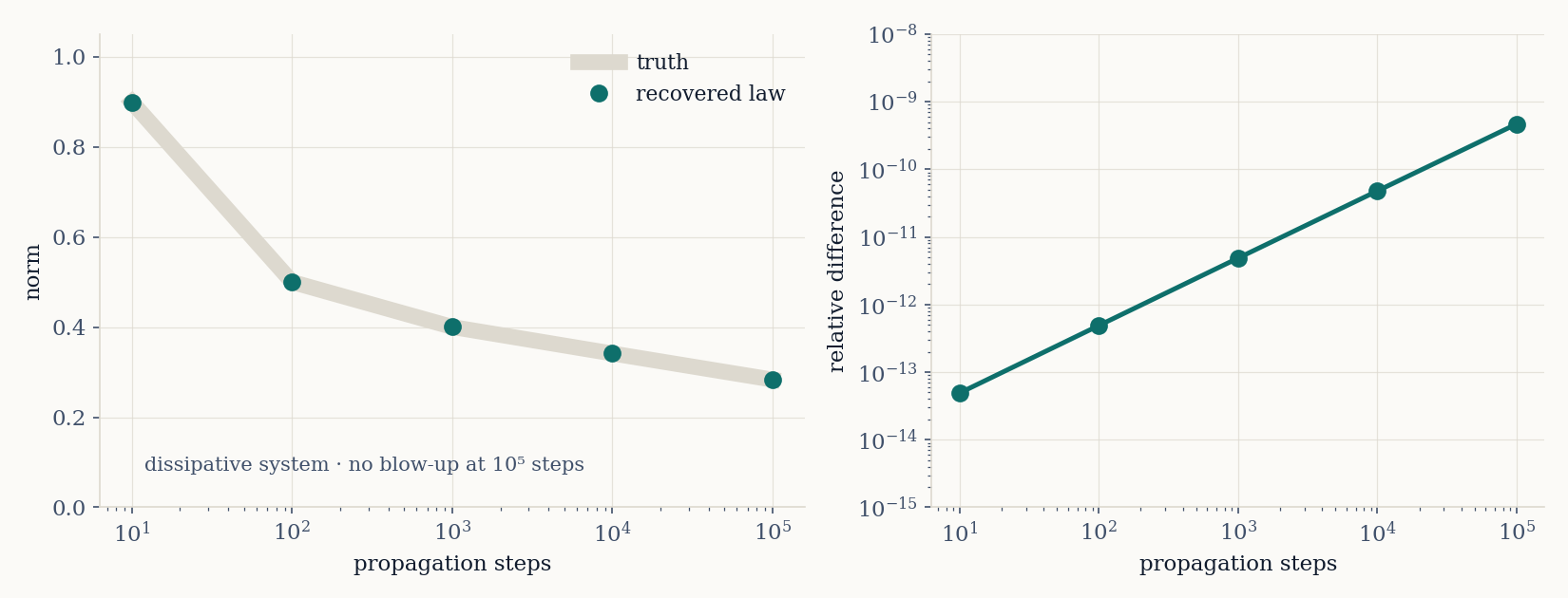
| Steps | True norm | Norm from the recovered law | Relative difference |
|---|---|---|---|
| 10 | 0.8991709 | 0.8991709 | 4.9×10⁻¹⁴ |
| 1 000 | 0.4002519 | 0.4002519 | 4.9×10⁻¹² |
| 10 000 | 0.3414142 | 0.3414142 | 4.8×10⁻¹¹ |
| 100 000 | 0.2834039 | 0.2834039 | 4.7×10⁻¹⁰ |
The last figure is the control: applying the isolated-system constraint to a dissipative system raises the error to 2.1×10⁻¹ — twelve orders of magnitude. The value lies not in projecting, but in knowing which projection. Damping rates separate correctly from energies, to 2.4×10⁻¹³.
We can say when and by how much a model will be wrong, before using it there
The certificate yields a rate. Calibrated on a single point, it predicts degradation across three orders of magnitude in the propagation horizon. For the reference, the same rate gives 1.000000 at any horizon — and that is what is measured.
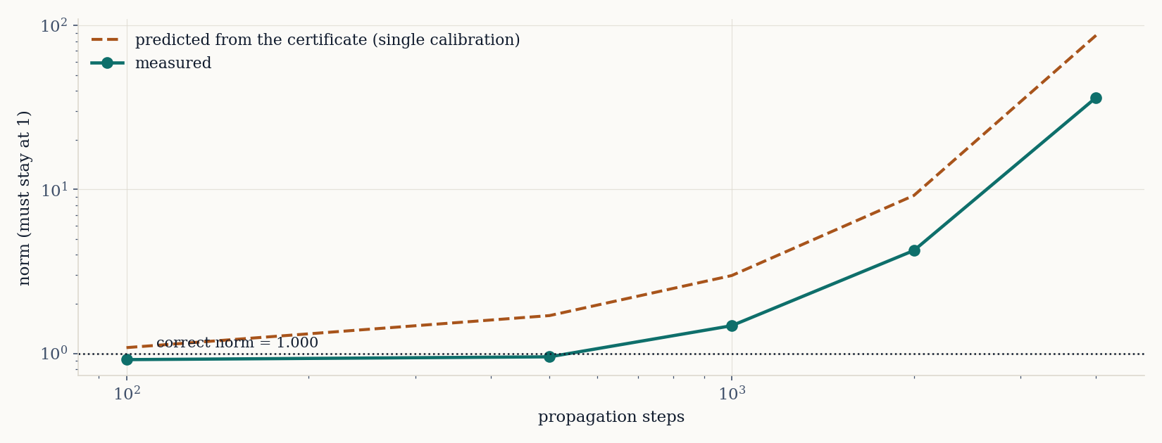
What the certificate catches
- The horizon beyond which prediction becomes unreliable.
- Regions of input space outside the domain of validity.
- The case where the model predicts well but the inferred law is false.
The two measured frontiers
- Temporal resolution. Sharp threshold to the fourth decimal. Below it the law is recovered exactly; above it prediction stays perfect while the law is false.
- Partial observability. Removing 5% of the domain destroys the structure entirely — thirteen orders. A threshold, not a slope.
- Noise is not a frontier. With structure exploited, parameters come out more than a hundred times more precise than the noise level.
The distinction that matters commercially: in two of five failure modes, prediction remains flawless while the recovered law is false. Any method that reports only prediction error cannot see this.
Accuracy decouples from problem size
Same physics, same target. The adapted representation reaches with 59 degrees of freedom an accuracy the conventional method does not reach at two million — and past an optimum it degrades.
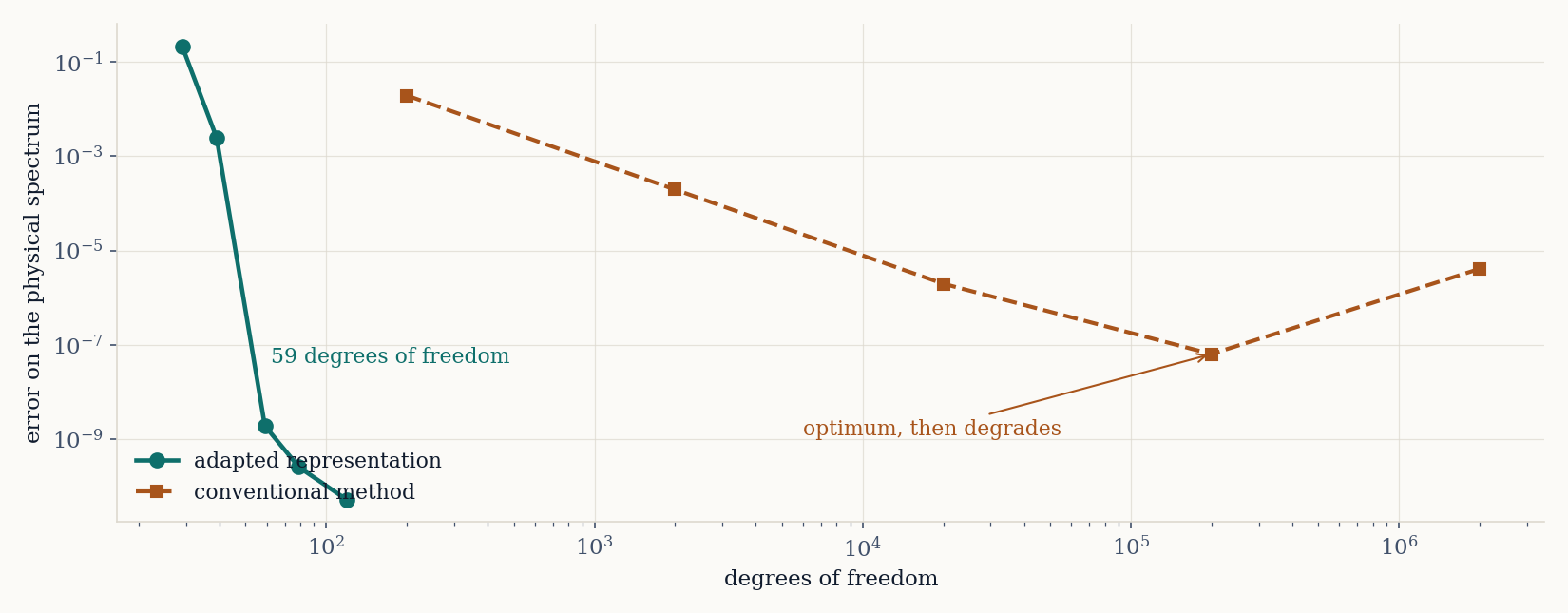
| Accuracy required | Conventional method | Adapted representation |
|---|---|---|
| 10⁻⁴ | 5 000 | 49 |
| 10⁻⁶ | 100 000 | 59 |
| 10⁻⁸ | over 8×10⁶ | 59 |
| 10⁻¹⁰ | over 8×10⁶ | 119 |
The two regimes are not a matter of preference: a discriminant measured on the data states unambiguously which one you are in. For problems where the physics genuinely requires many degrees of freedom, the sparse route handles a million in 1.5 seconds on a single core.
Where each result applies, and what it requires
Conditions of validity
- The dynamics must be linear in the state — this covers quantum mechanics, electromagnetism, diffusion, linear acoustics, and any system linearised about an operating regime.
- For nonlinear dynamics the audit applies on the tangent space; the required representation has been identified and validated.
- The temporal resolution of the data must satisfy an explicit sampling condition, verifiable before any run.
- Spatial observability must be complete; partial loss is detected rather than hidden.
Immediate extensions
- Audit-as-a-service for dynamics models already in production — no code access required.
- Sizing the data budget ahead of expensive acquisition campaigns.
- Instrumentation time series, where no standardised refusal criterion exists.
| Sector | What is gained | Applicable result |
|---|---|---|
| Simulation surrogates | A physics certificate; grounded refusal instead of silent extrapolation | 2, 5, 10, 11 |
| Measurement campaigns | The number of examples, computed in advance | 1, 6 |
| System identification | The law and its structure, from short trajectories | 3, 4, 8, 9 |
| High-fidelity computation | Accuracy decoupled from grid size | 12 |